Neuroscience Basic Knowledge

The LIF model

LIF: Leaky Integrated-and -Fire

1. Membrane Equation

$$ \begin{align*} \
&\tau_m\,\frac{d}{dt}\,V(t) = E_{L} - V(t) + R\,I(t) &\text{if }\quad V(t) \leq V_{th} \\
\\
&V(t) = V_{reset} &\text{otherwise}\
\
\end{align*} $$

where $V(t)$ is the membrane potential(膜电势), $\tau_m$ is the membrane time constant, $E_{L}$ is the leak potential, $R$ is the membrane resistance, $I(t)$ is the synaptic input current, $V_{th}$ is the firing threshold, and $V_{reset}$ is the reset voltage. We can also write $V_m$ for membrane potential, which is more convenient for plot labels.

The membrane equation describes the time evolution of membrane potential $V(t)$ in response to synaptic input and leaking of charge across the cell membrane. This is an ordinary differential equation (ODE).

2. Reset Condition

A spike takes place whenever $V(t)$ crosses $V_{th}$. In that case, a spike is recorded and $V(t)$ resets to $V_{reset}$ value. This is summarized in the *reset condition*: $$V(t) = V_{reset}\quad \text{ if } V(t)\geq V_{th}$$

3. Refractory Period

$refractory period plot$

The absolute refractory period is a time interval in the order of a few milliseconds during which synaptic input will not lead to a 2nd spike, no matter how strong.

4. Python Code for Simulating a LIF Neuron

# Simulation class
class LIFNeurons:
  """
  Keeps track of membrane potential for multiple realizations of LIF neuron,
  and performs single step discrete time integration.
  """
  def __init__(self, n, t_ref_mu=0.01, t_ref_sigma=0.002,
               tau=20e-3, el=-60e-3, vr=-70e-3, vth=-50e-3, r=100e6):

    # Neuron count
    self.n = n

    # Neuron parameters
    self.tau = tau        # second
    self.el = el          # milivolt
    self.vr = vr          # milivolt
    self.vth = vth        # milivolt
    self.r = r            # ohm

    # Initializes refractory period distribution
    self.t_ref_mu = t_ref_mu
    self.t_ref_sigma = t_ref_sigma
    self.t_ref = self.t_ref_mu + self.t_ref_sigma * np.random.normal(size=self.n)
    self.t_ref[self.t_ref<0] = 0

    # State variables
    self.v = self.el * np.ones(self.n)
    self.spiked = self.v >= self.vth
    self.last_spike = -self.t_ref * np.ones([self.n])
    self.t = 0.
    self.steps = 0


  def ode_step(self, dt, i):

    # Update running time and steps
    self.t += dt
    self.steps += 1

    # One step of discrete time integration of dt
    self.v = self.v + dt / self.tau * (self.el - self.v + self.r * i)

    # Spike and clamp
    self.spiked = (self.v >= self.vth)
    self.v[self.spiked] = self.vr
    self.last_spike[self.spiked] = self.vr
    clamped = (self.last_spike + self.t_ref > self.t)
    self.v[clamped] = self.vr

    self.last_spike[self.spiked] = self.t

# Set random number generator
np.random.seed(2020)

# Initialize step_end, t_range, n, v_n and i
t_range = np.arange(0, t_max, dt)
step_end = len(t_range)
n = 500
v_n = el * np.ones([n, step_end])
i = i_mean * (1 + 0.1 * (t_max / dt)**(0.5) * (2 * np.random.random([n, step_end]) - 1))

# Initialize binary numpy array for raster plot
raster = np.zeros([n,step_end])

# Initialize neurons
neurons = LIFNeurons(n)

# Loop over time steps
for step, t in enumerate(t_range):

  # Call ode_step method
  neurons.ode_step(dt, i[:,step])

  # Log v_n and spike history
  v_n[:,step] = neurons.v
  raster[neurons.spiked, step] = 1.

# Report running time and steps
print(f'Ran for {neurons.t:.3}s in {neurons.steps} steps.')

# Plot multiple realizations of Vm, spikes and mean spike rate
plot_all(t_range, v_n, raster)

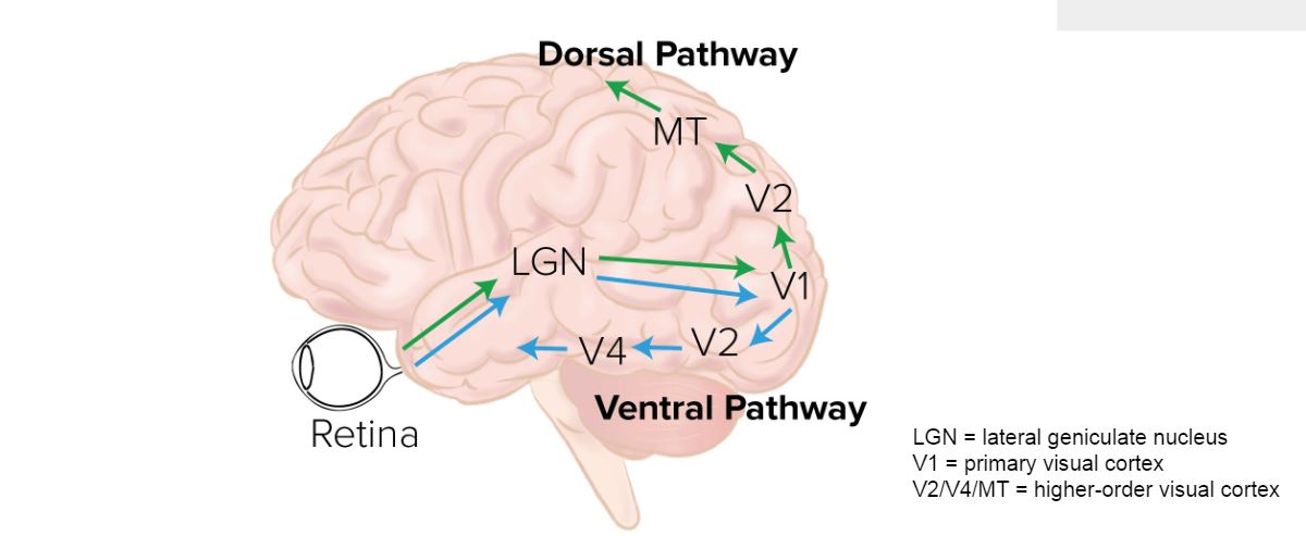
The Mammalian Visual System

1. Structure

Estimating receptive fields: spike-triggered averaging(STA)

Brandon Zhang