Classification
Classification
I. Probabilistic Generative Models
1. Detailed Process
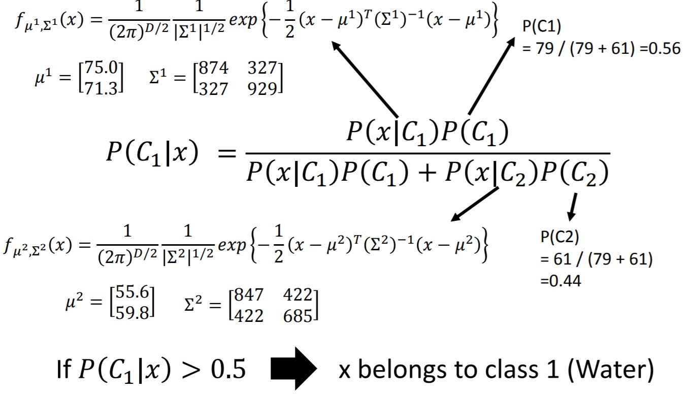
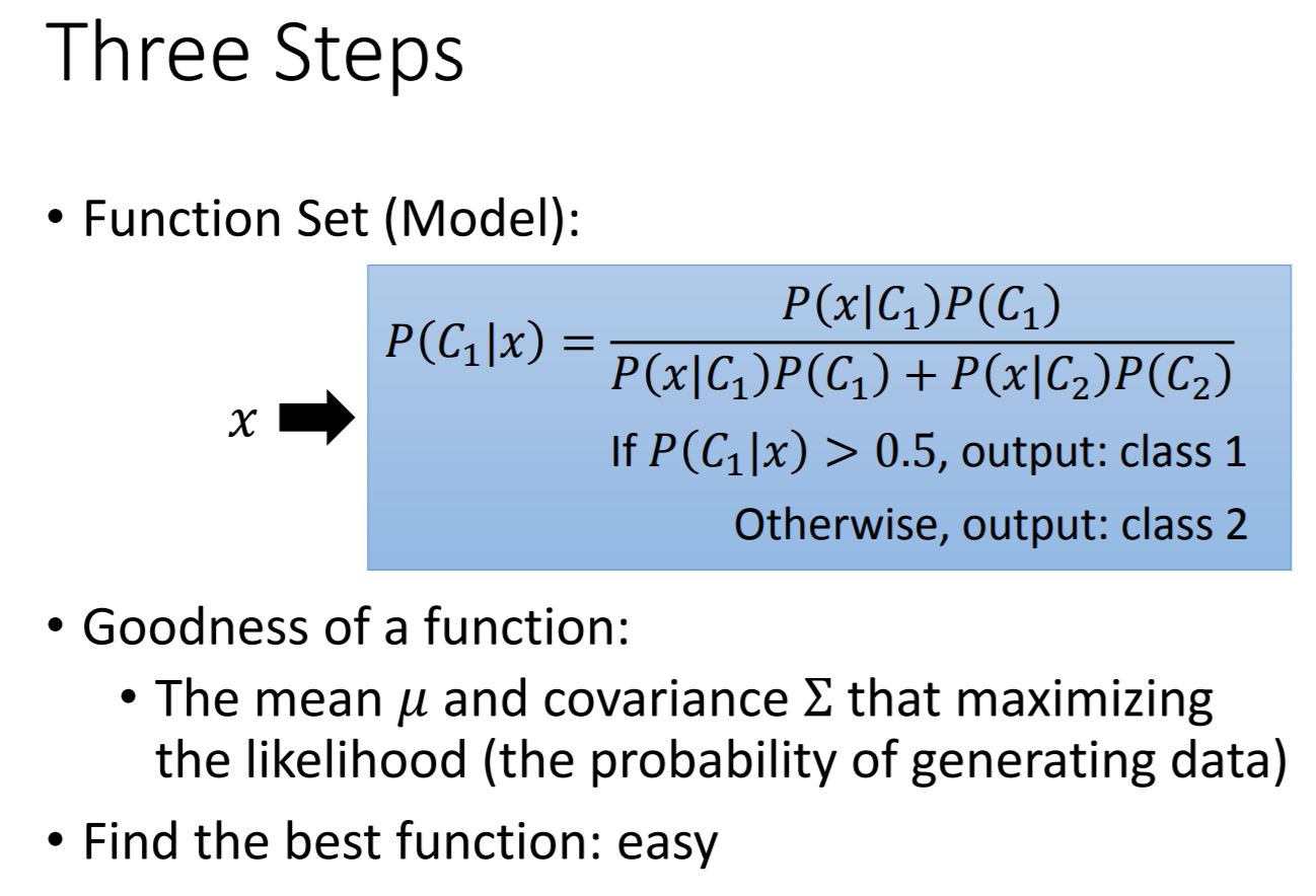
The basic idea is estimating the probabilities form training data. Let’s consider the two classes case:
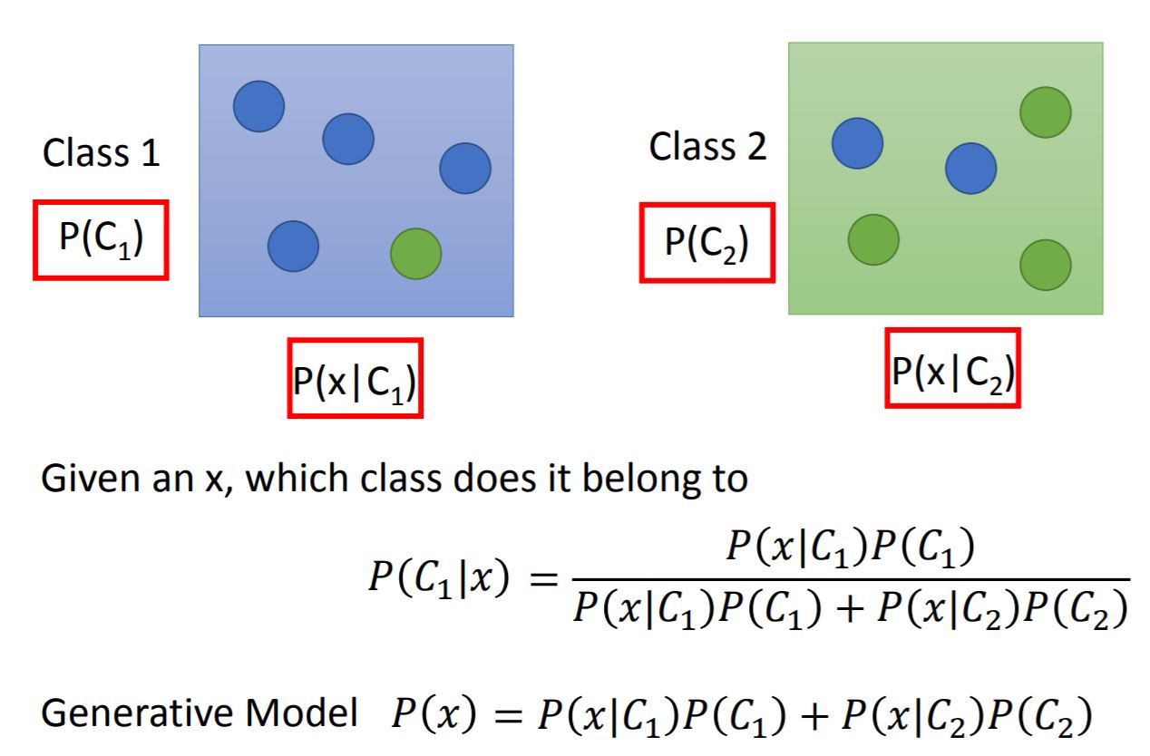

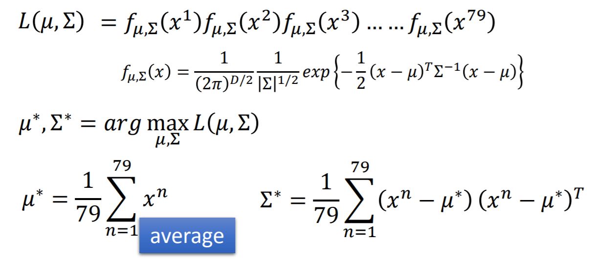
2. Modifying Model
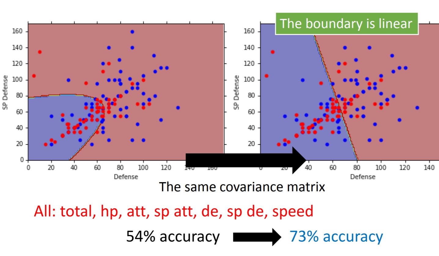
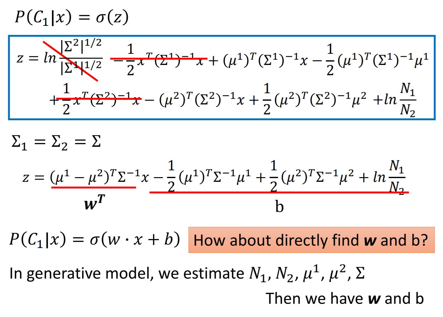
While we are training the model, we normally choose the same covariance matrix $\Sigma$ for each Gaussian Distribution. The reason for doing this is to have less parameters for the training model, also from the result we can see the accuracy has increased (Maybe just in this case).
3. Summary
4. Tips
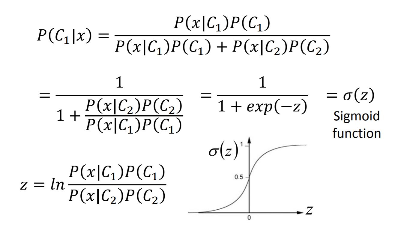
- Posterior Probability & Sigmoid function
- Posterior Probability & Logistic Regression
II. Logistic Regression
1. Detailed Process
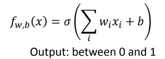
Step 1: Function Set
Step 2: Goodness of Function
Cross entropy (交叉熵) : 如果两个分布相同,则交叉熵为0。In logistic regression we have training data $(x^n, \hat{y}^n)$, where $\hat{y}^n$: 1 for class 1, 0 for class 2.

Step 3: Gradient Descent
The update function of parameter $\omega$ is:
2. Discriminative vs Generative
- The benefits of Generative model
- With the assumption of probability distribution, less training data is needed;
- With the assumption of probability distribution, more robust to the noise;
- Priors and class-dependent probabilities can be estimated from different sources.
关于第三点需要着重解释一下。对于大部分神经网络都是判别模型,这种模型也确实会有更高的准确率。但对于类似语音识别的task中,priors和class-dependent probabilities是可以分开计算的,例如先验概率是由海量的网上数据计算而得,而class-dependent probabilities是根据语音数据计算得来。
3. Multi-class Classification
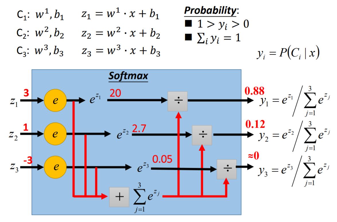
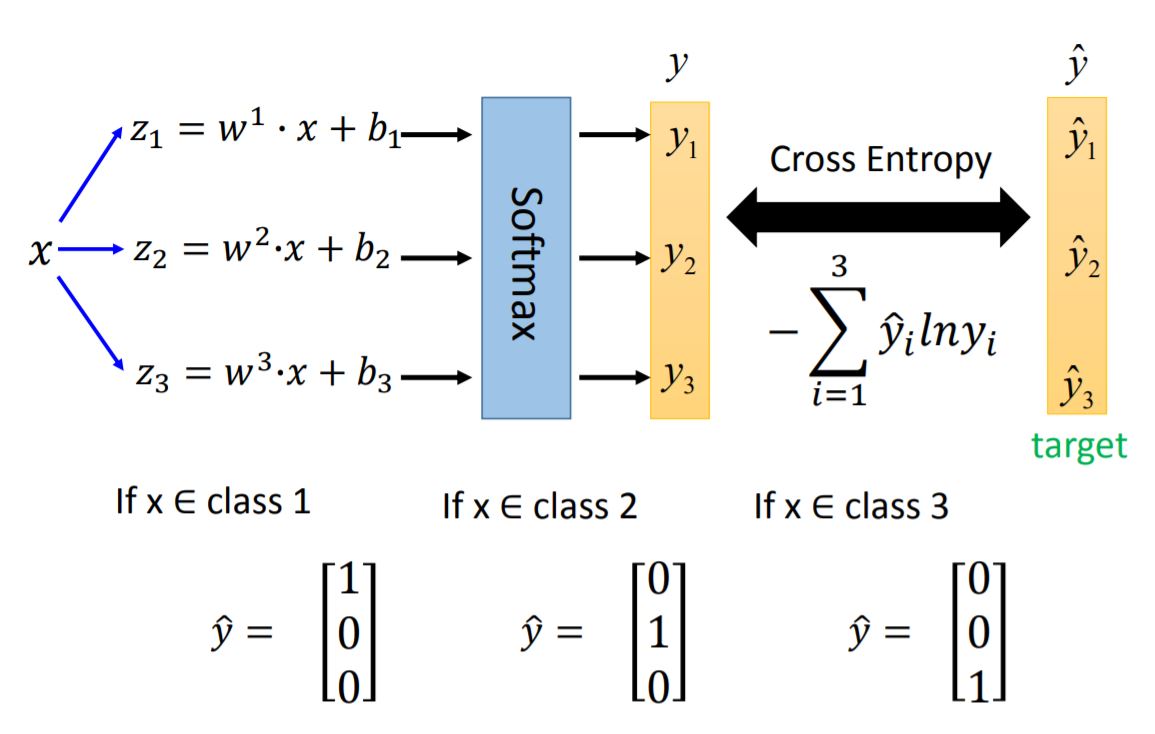
4. Limitation of Logistic Regression
XOR Problem can’t be solved by Logistic Regression.
Solution
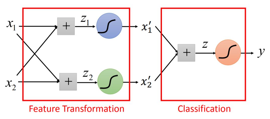
Feature Transformation It’s not always easy to find a good transformation. (与SVM中的Kernel函数类似)
Cascading logistic regression models 中间的变换为分线性变换,使得在后续可分。

