
Brandon Zhang
July 25, 2020
Optimization for Deep Learning
Some Notation: $\theta_t$: model parameter at time step t $\nabla$$L(\theta_t)$ or $g_t$: gradient at $\theta_t$, used to compute $\theta_{t+1}$ $m_{t+1}$: momentum accumlated from time step 0 to time step t, which is used to compute $\theta_{t+1}$
I. Adaptive Learning Rates
In gradient descent, we need to set the learning rate to converge properly and find the local minima. But sometimes it’s difficult to find a proper value of the learning rate. Here are some methods to introduce which can automatically produce the adaptive learning rate based on the certain situation.
- Popular & Simple Idea: Reduce the learning rate by some factor every few epochs (eg. $\eta^t=\eta/\sqrt{t+1}$)
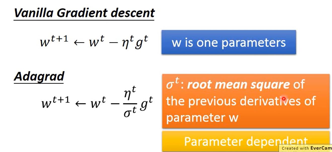
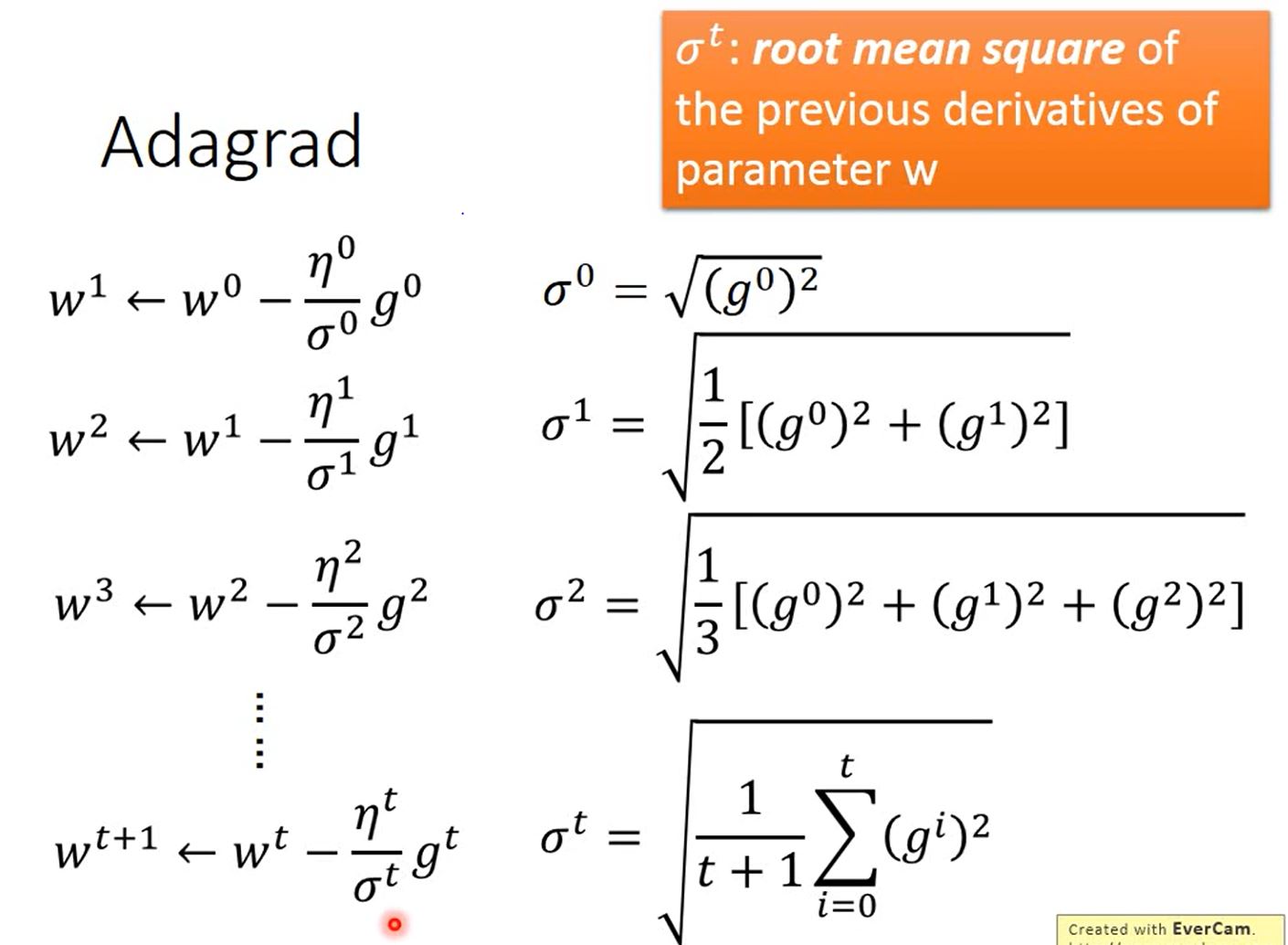
- Adagard: Divide the learning rate of each parameter by the root mean square of its previous derivatives
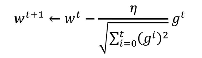
 When $\eta = \frac{\eta^t}{\sqrt{t+1}}$, we could derive that:
II. Stochastic Gradient Descent
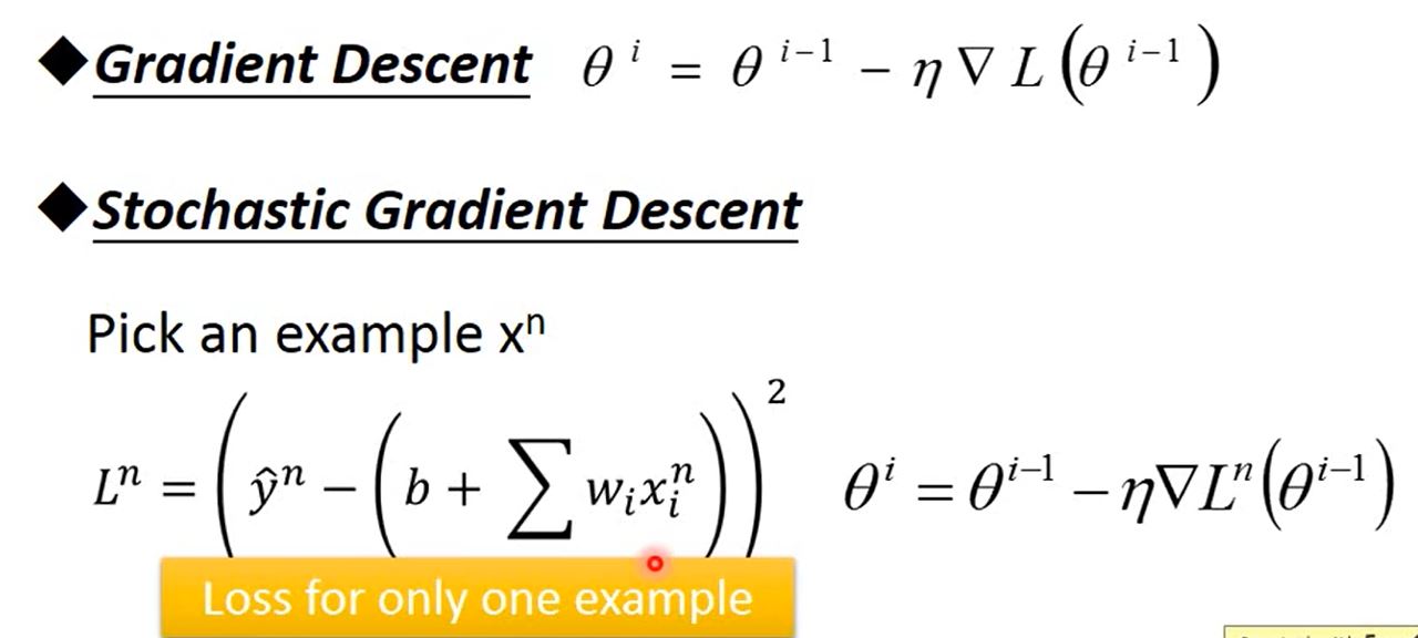 SGD update for each example, so it would converge more quickly.
III. Limitation of Gradient Descent
- Stuck at local minima ($\frac{\partial L}{\partial \omega}$ = 0)
- Stuck at saddle point ($\frac{\partial L}{\partial \omega}$= 0)
- Very slow at plateau: Actually this is the most serious limitation of Gradient Descent.
So there are other methods perform better than gradient descent.
IV. New Optimizers
notice: on-line: one pair of ($x_t$, $\hat{y_t}$) at a time step off-line: pour all ($x_t$, $\hat{y_t}$) into the model at every time step
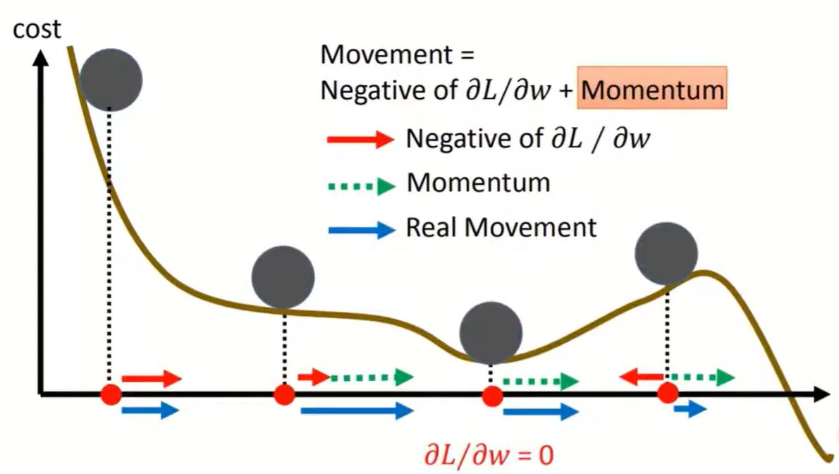
1. SGD with Momentum (SGDM)
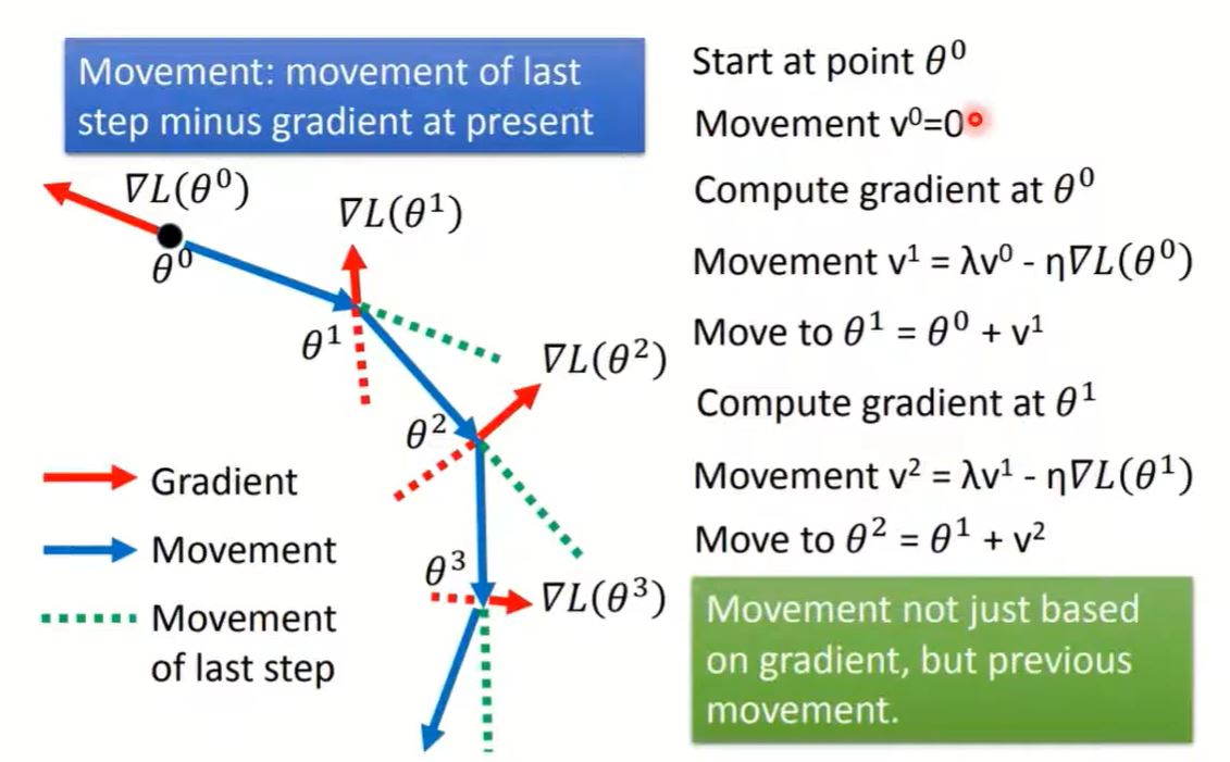 Previous gradient will affect the next movement. $v^i$ is actually the weighted sum of all the previous gradient:
$\nabla L(\theta^0), \nabla L(\theta^1), \dots \nabla L(\theta^{i-1})$
Use SGDM could erase the limitation of $\nabla L(\theta) = 0$.
For momentum, you could imagine it as physical inertia.
Previous gradient will affect the next movement. $v^i$ is actually the weighted sum of all the previous gradient:
$\nabla L(\theta^0), \nabla L(\theta^1), \dots \nabla L(\theta^{i-1})$
Use SGDM could erase the limitation of $\nabla L(\theta) = 0$.
For momentum, you could imagine it as physical inertia.
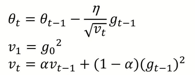
2. Root Mean Square Propagation (RMSProp)
This optimizer is based on Adagrad, but the main difference is the calculation of the denominator. The reason for this new calculation is to avoid the situation that the learning rate is too small from the first step. In other words, exponential moving average(EMA) of squared gradients is not monotonically increasing.
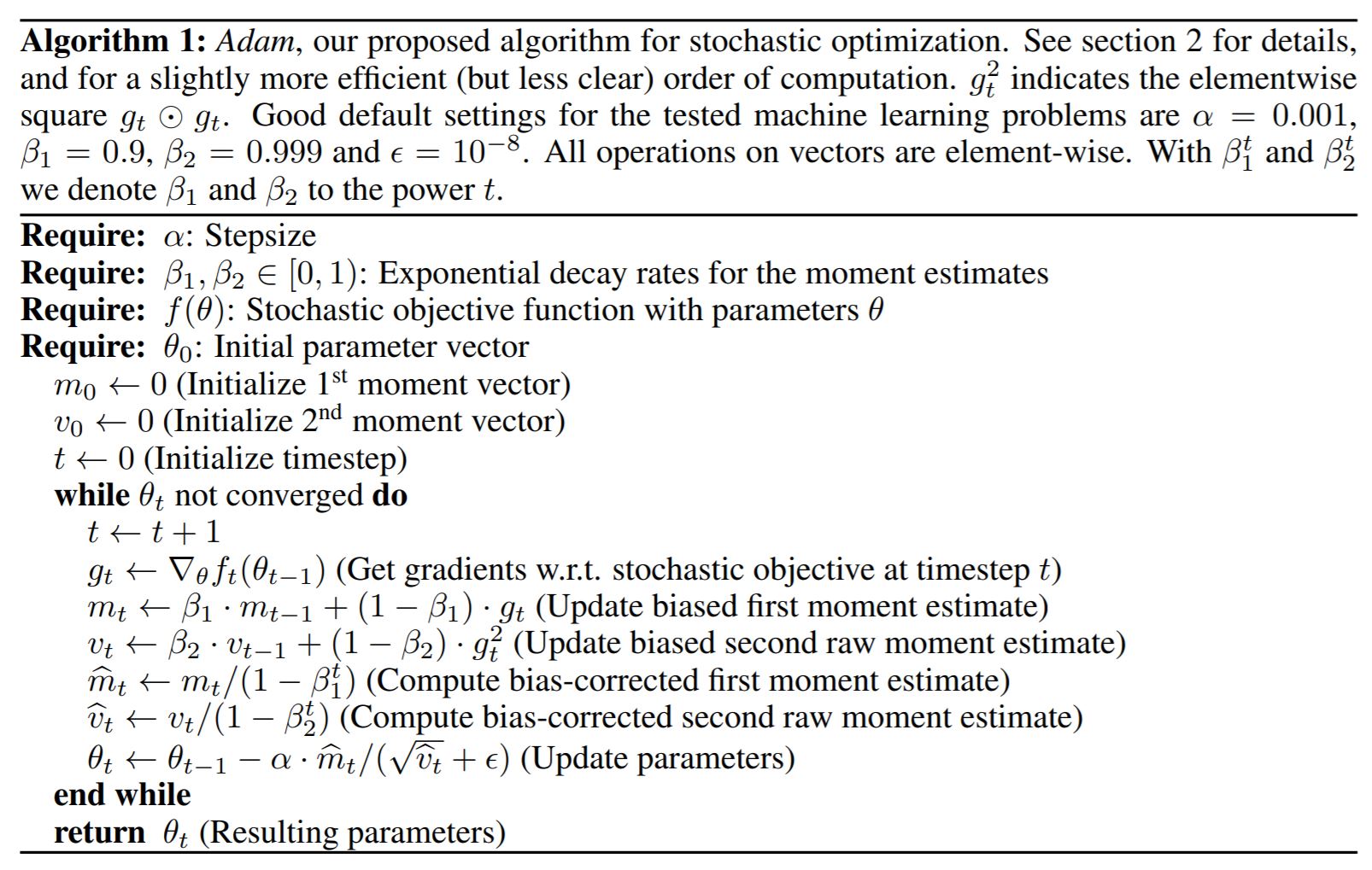
3. Adam
Adam is an optimization algorithm that can be used instead of the classical stochastic gradient descent procedure to update network weights iterative based in training data.
Adam realizes the benefits of both AdaGrad and RMSProp.
4. Adam vs SDGM
- Adam: fast training, large generalization gap, unstable
- SGDM: stable, little generalization gap, better convergence
5. Supplement
ASMGrad (ICLR'18)
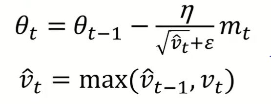
AdaBound (ICLR'19)
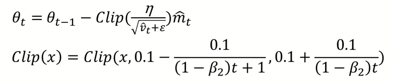
note: Clip(x, lowerbound, upperbound)
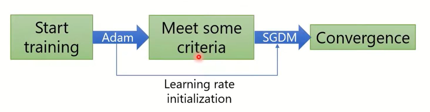
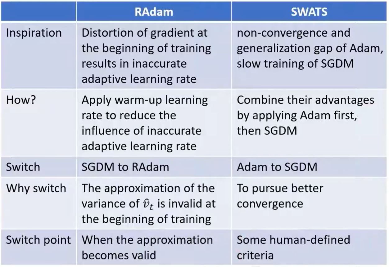
SWATS (arXiv'17) Begin with Adam(fast), end with SGDM
RAdam (Adam with warmup, ICLR'20)
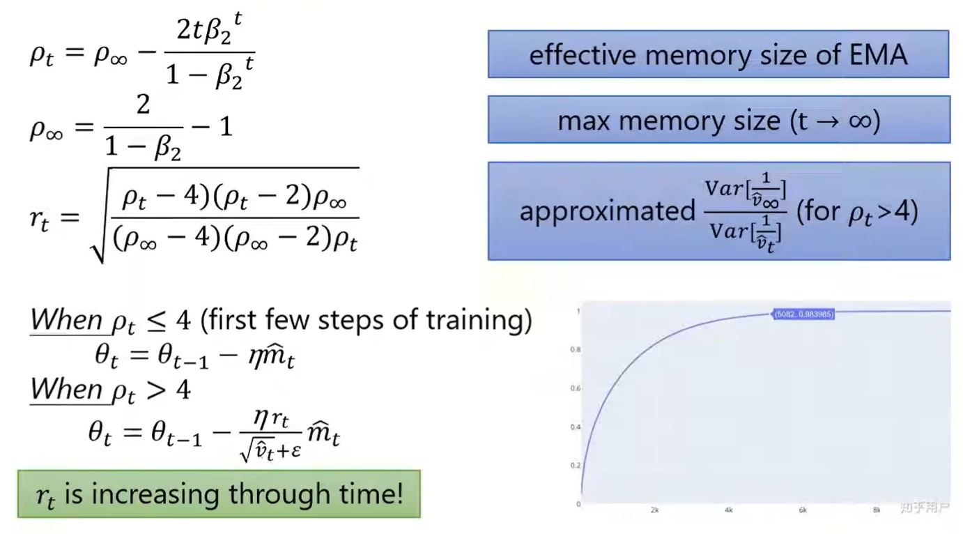
RAdam vs SWATS
To be continued …