
Brandon Zhang
August 10, 2020
Introduction to Deep Learning
I. Basic Concepts
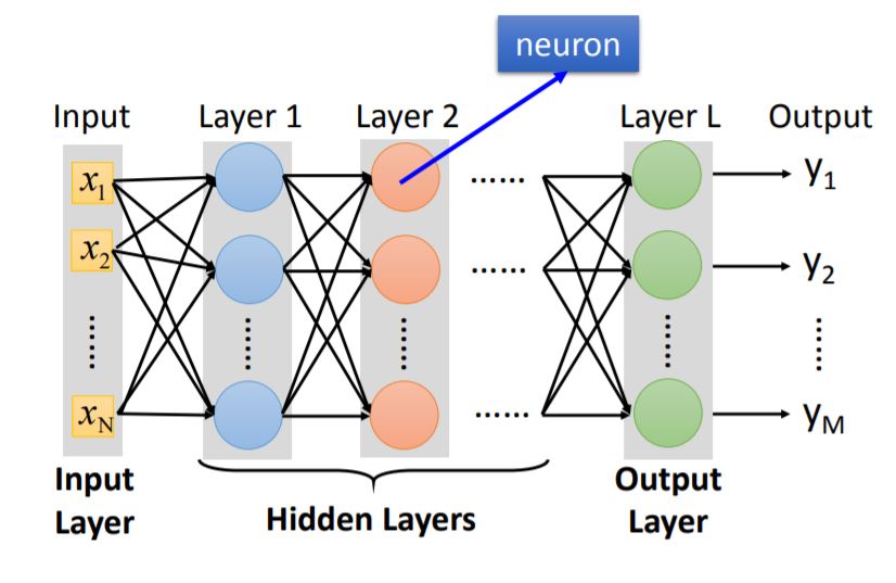
1. Fully Connected Feedforward Network
2. Matrix Operation
Every layer has weight matrix and bias matrix, using matrix operation we can accumulate the output matrix $y$.
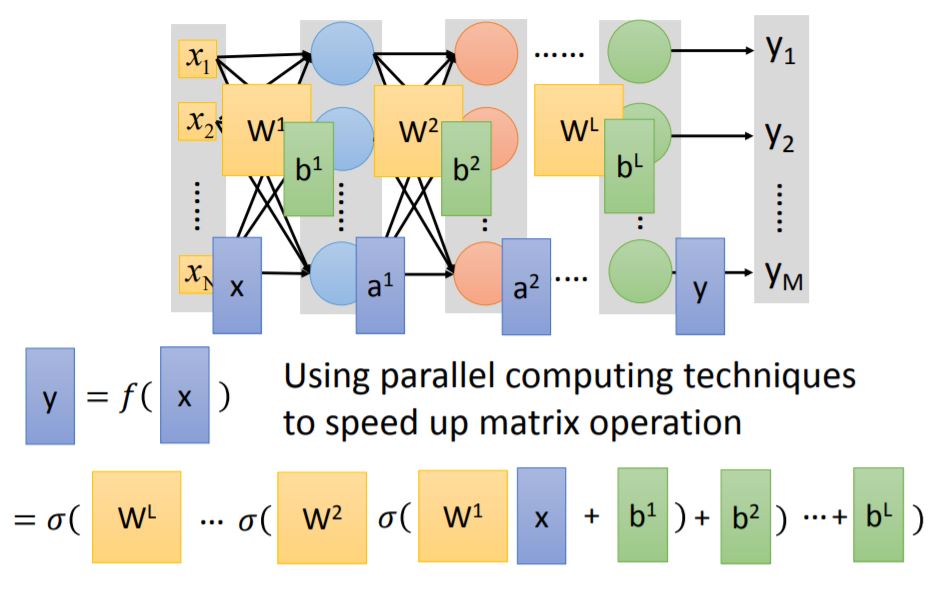
Tips: Using GPU could speed up matrix operation.
II. Why Deep Learning?
1. Modularization
对neural network而言,并不是神经元越多越好,通过例子可以看出层数的增加(more deep)对于准确率的提升更有效果。这其中就是 Modularization 的思想。
For example, while you are trying to train the model below, you can use basic classifiers as module. Each basic classifier can have sufficient training examples. Therefore those classifiers can use output from the basic classifiers, which can be trained by little data.
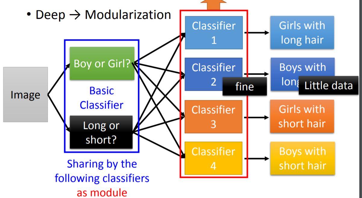 What you should notice is that the modularization is automatically learned form data.
III. Backpropagation
1. Concept
An Efficient way to compute gradient descent $\partial{L}/\partial{\omega}$ in neural network.
2. Detailed Process
The partial of the loss function can be presented as follow:
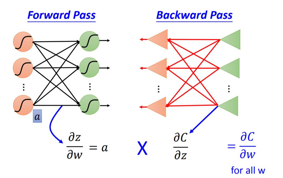
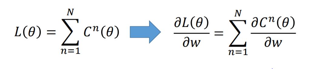 According to Chain rule, we need to compute two partials: Forward pass and Backward pass.
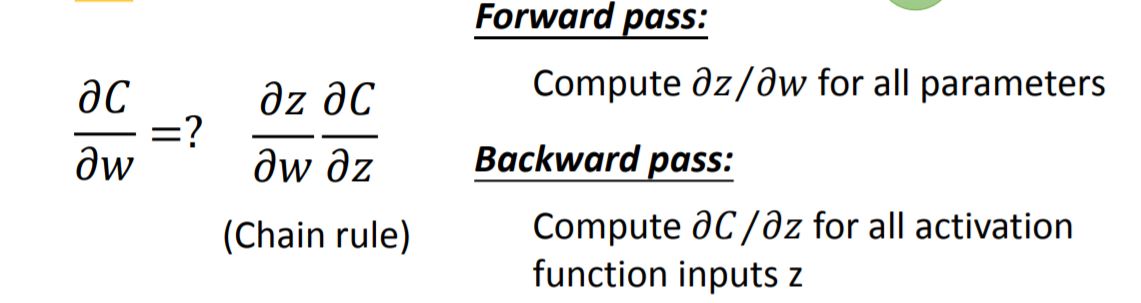
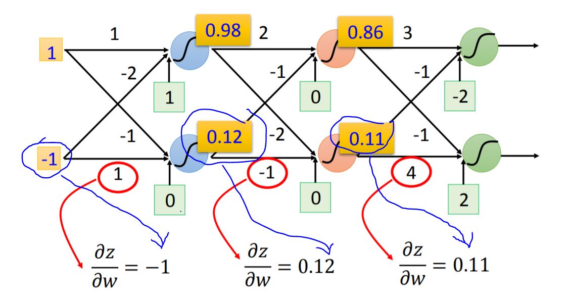
Forward pass $\partial{z}/\partial{\omega} = $ The value of the output connected by the weight.
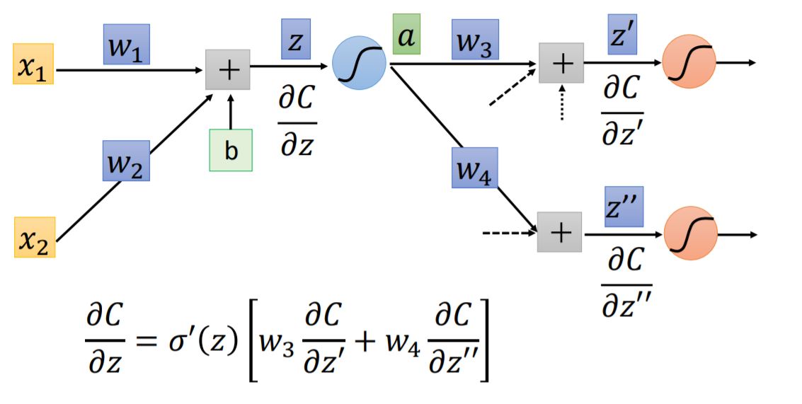
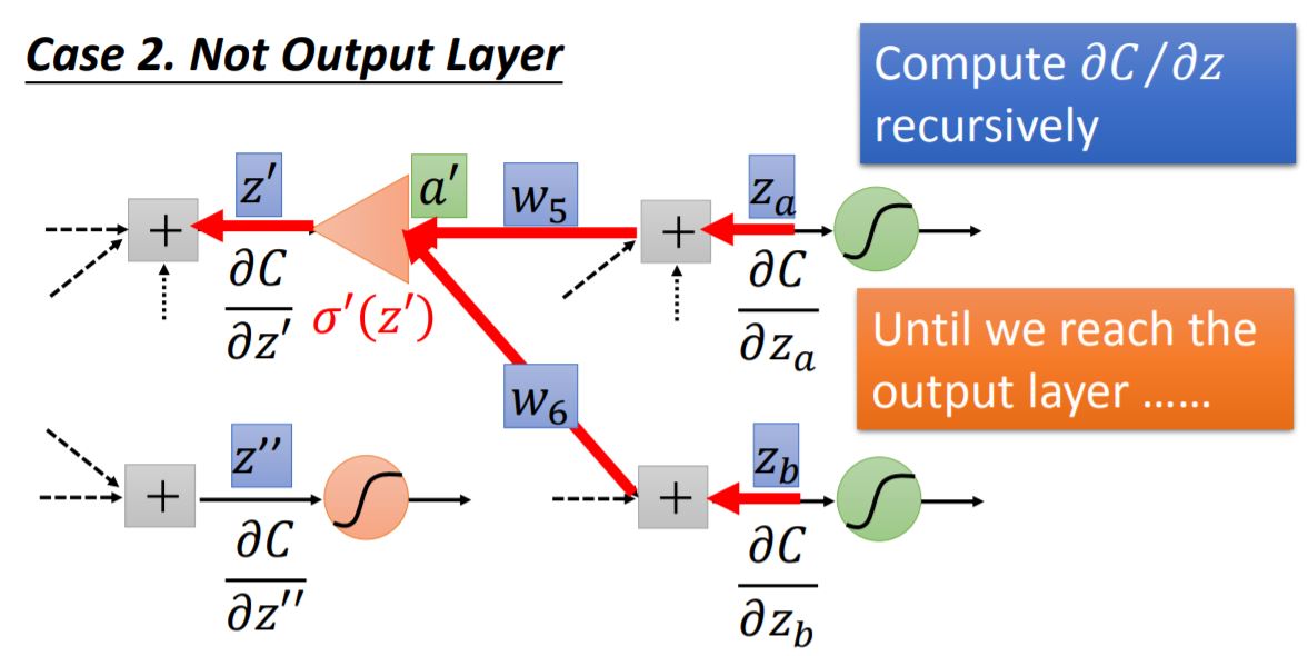
Backward pass To compute $\partial{C}/\partial{z}$, we need to figure out following neurons' partial.
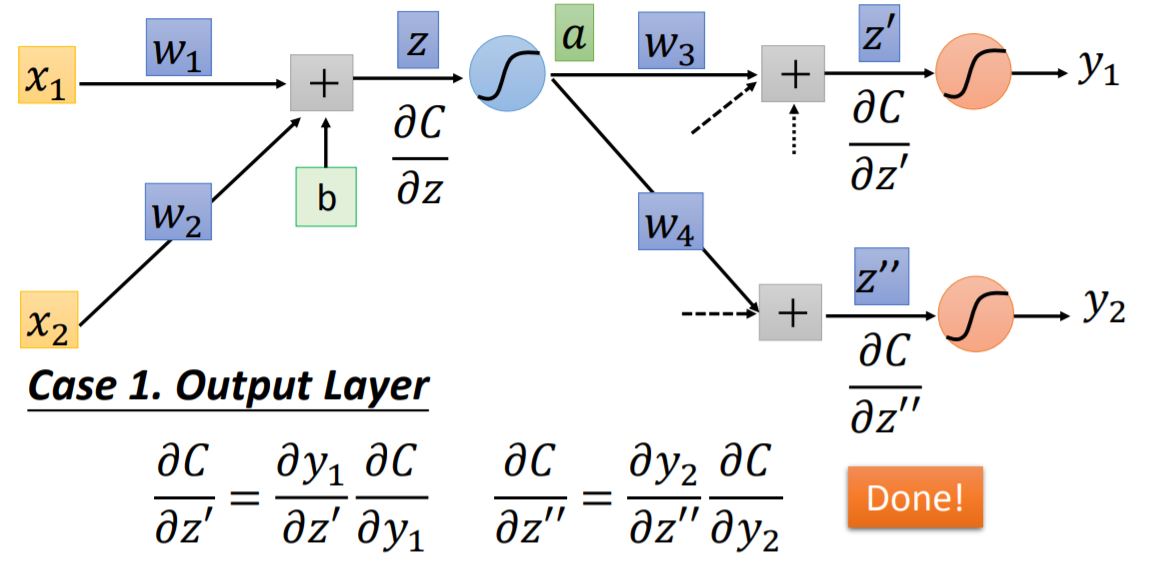
case 1: Output Layer When we arrive at the output layer of the network, these two partials: $\partial{C}/\partial{z'} = \partial{C}/\partial{y_1}$ and $\partial{C}/\partial{z''} = \partial{C}/\partial{y_2}$ could be solved pretty easy.
case 2: Not Output Layer We could compute $\partial{C}/\partial{z}$ recursively, until we reach the output layer. Then we start to backward pass. It seems like a new backward neural network (red line in the graph).
The whole process of backpropogation is shown as following graph:
IV. Tips for DL
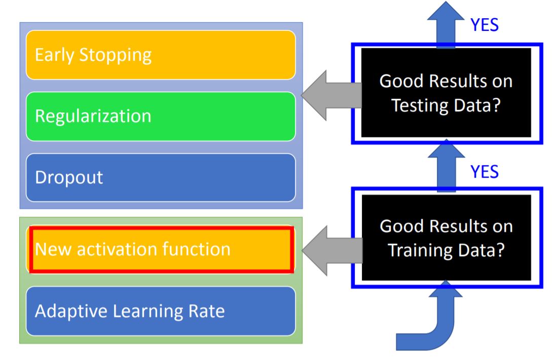
1. New activation function
- Vanishing Gradient Descent
This phenomenon is mainly caused by the particular activation function: sigmoid funcion.
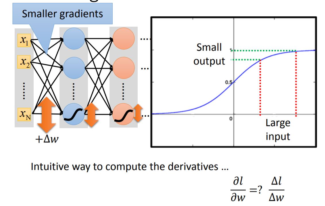 From the analysis above when given a large $\Delta{\omega}$ as an input, the output from sigmoid function is become smaller. After going through many layers, the gradient goes to a small value, also called vanished.
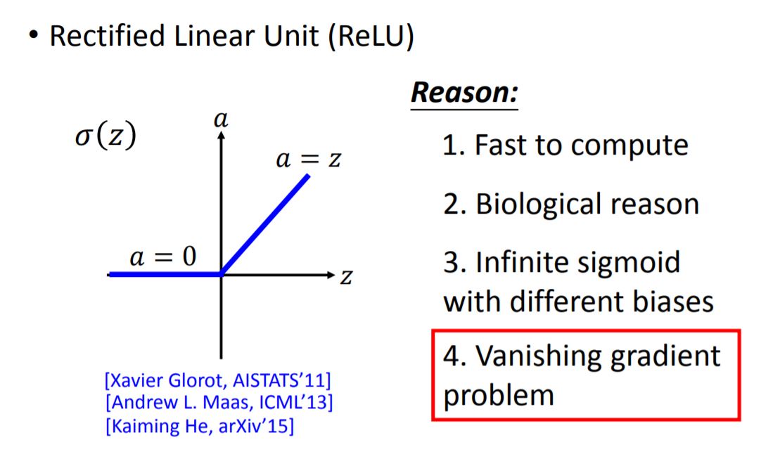
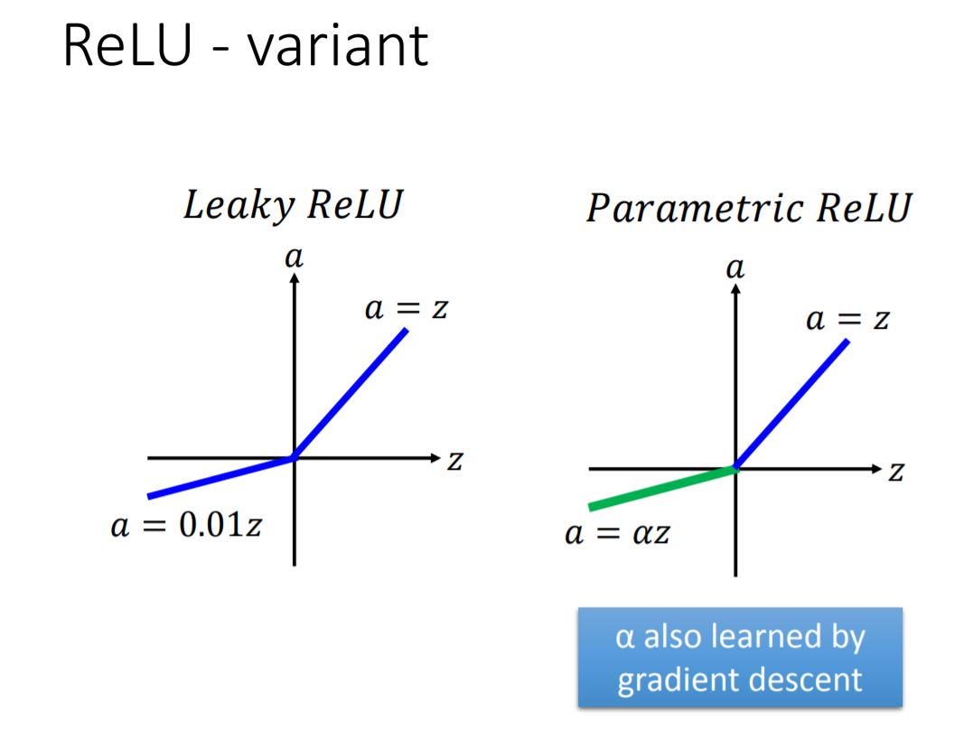
(1) ReLU
(2) Maxout
ReLU is a special case of Maxout
For Maxout function, we can design the form of activation funcion by our own.

- Activation function in maxout network can be any piecewise linear convex function
- How many pieces depending on how many elements in a group
Question 1: How to train Maxout network?
Answer: 对于每一个神经元,他们先比大小取出较大$z_i$作为输入,再将其对应的linear function拿去作微分
Quesion 2: 有些output被舍去之后,back propogation无法再对其进行训练?
Answer: We can train different thin and linear network for different example.
2. Adaptive Learning Rate
tips: 实际上对于local minima, 并不会存在过多,local minima的出现需要每一个dimension在附近都会产生local minima。假设一个dimension在这里出现local minima的概率为p,由于神经网路需要非常多的parameters,local minima出现的概率很低。
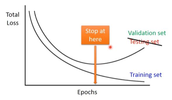
3. Early Stopping
Using Validation Set to simulate testing set, then we could find where to stop properly.
4. Regularization
New loss function to be minimized:
- Find a set of weight not only minimizing original cost but also close to zero.
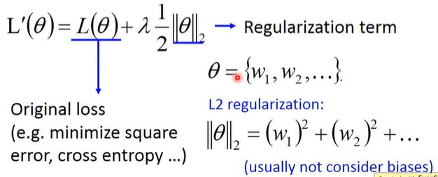
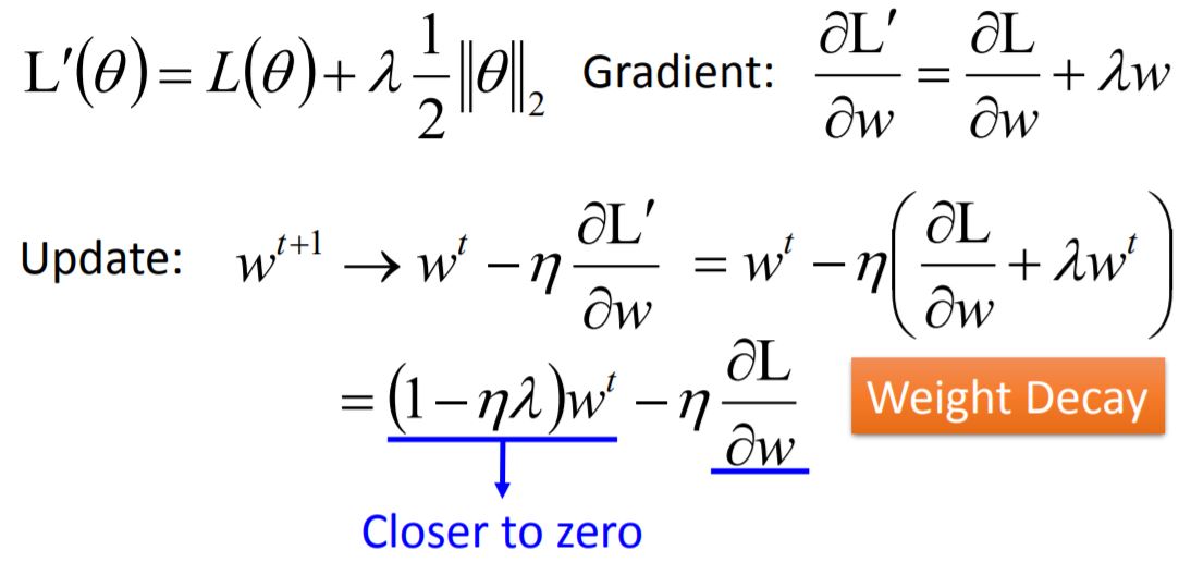
- L2 regularization (二范数)
Weight Decay (权重衰减) 对于一些长期不需要用到的weight,它的值会随着训练次数接近0,这种模式接近于人脑神经元的构造方式。
- L1 regularization
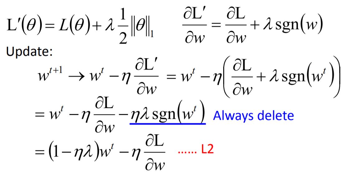 L1 每次减掉固定的值,使得每次迭代后保留很多较大的值,得到的结果会比较稀疏,有很多接近于0,也有很多较大的值;然而对于L2,平均值较小。
5. Dropout
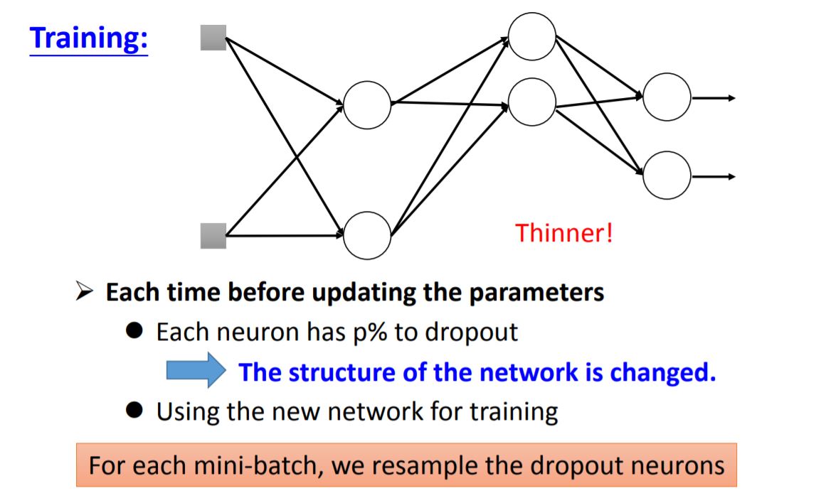
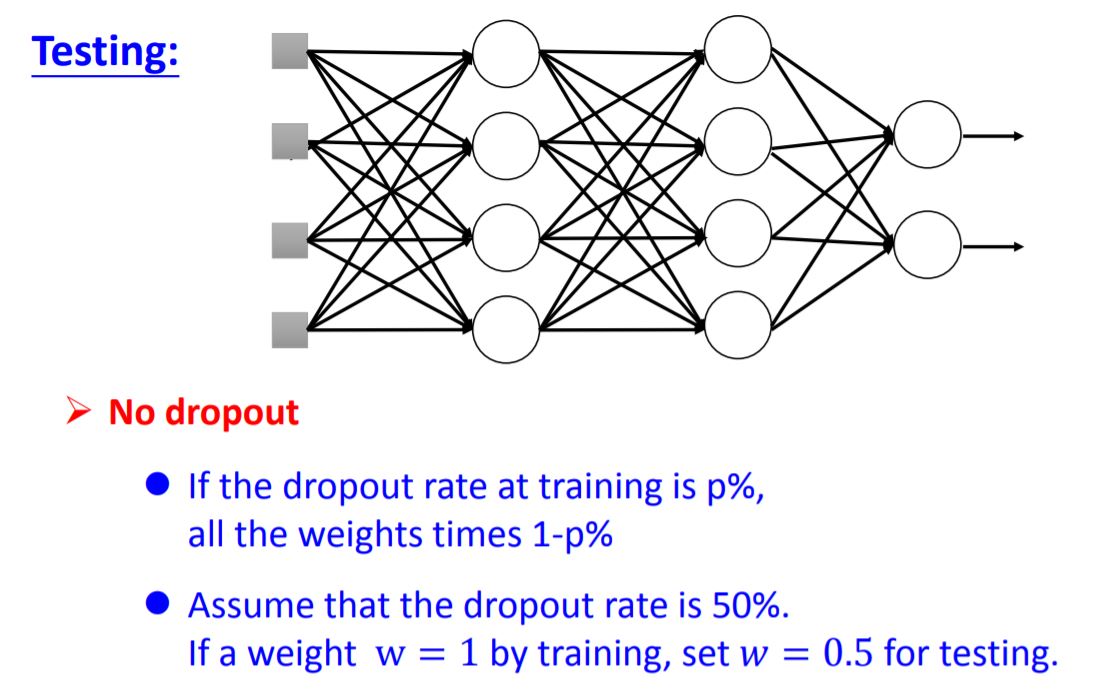 The amazing point of dropout:
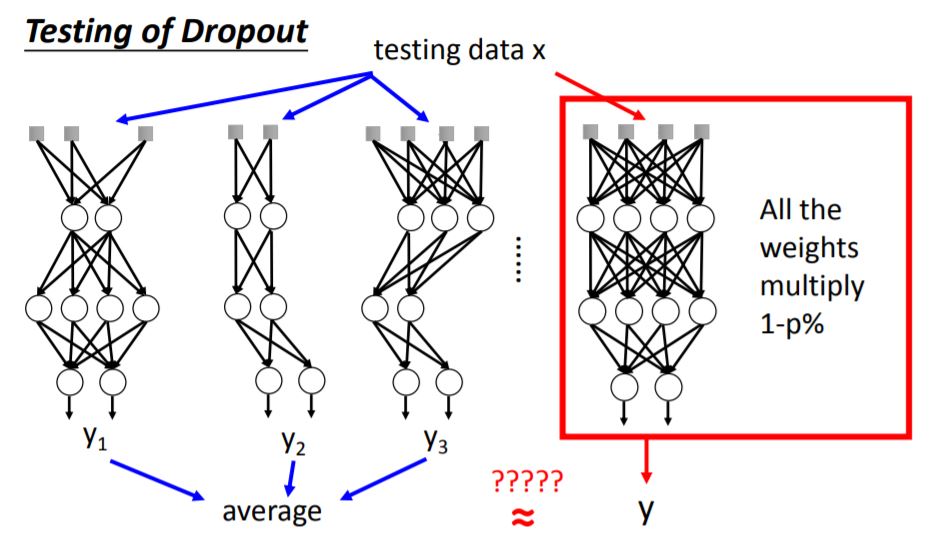
当你将测试集送入每一个minibatch训练的neural network,再将所有output求average,结果跟将测试集送入完整(未dropout,将所有weight乘以1-p%)的neural network得出来的结果是近似的。这点在线性模型中很容易解释,但对于非线性模型依旧有这个特性。所以Relu+dropout和Maxout+dropout的效果都会不错。